Step-by-step protocol for data collection using MISTRAL transmission X-ray microscope (TXRM): MISTRAL_Manual
On-sita data analysis
In-house software: Package with a command line interface. While your data is being collected there are a series of data analysis programs that are run at MISTRAL PC:
For spectroscopy data analysis
- To produce the E stack: energyscan --txm Escan.txt --stack
- Stack (to be done at a BL PC, with XMController software):
- XMController/File/Create .txrm from xrm
- add: select all files from spectrum (not FF! and not Add directory) & click once on 'File name' at top of window in order to organize files by Energy/name & create
- repeat for FF (when creating, better to give the same name as before adding _FF)
- From a linux computer and within the data folder (e.g. opbl09@pcbl0903:/> cd beamlines/bl09/projects/cycle2021-I/2021024878-laballe/DATA/20210424):
- Convert: txrm2nexus filename.txrm filename_FF.txrm
- Normalize: normalize filename.hdf5 -s=1
For alignment:
- xpy_tilt_align_h5 -i xxx_specnorm.hdf5:/SpecNormalized/spectroscopy_normalized -o xxx_spectnorm_aliOF –-ref 0
- ctalign filename_specnorm.hdf5 -s=1 -r=1
- Convert transmission to absorbance (A = -ln(T)), split the stack in single images (required for TXMWizard software), and include measured photon energy (Eenc) in each filename:
- (Optional) Copy aligned stack to a separate folder before splitting and obtaining ln.
- mkdir Newfoldername
- cp filename_specnorm_ali.hdf5 Newfoldername
- splithdfln filename_specnorm_ali.hdf5
- TXMWizard/TXM E Scan/TXM-XANES Wizard. Load/Load Image Stack: select all split images
- Tools/Crop images: rectangular selection excluding detector edges for ALL the series (check end ones!). Once selected, double click to apply.
- Press either Get bulk XANES or Get XANES of ROI for a first spectrum. Former will average all image, latter requires a post selection with the mouse (painting without lifting & at the end double-click).
- Select points (at least a few, if possible tens) from spectrum corresponding to pre-edge and to post-edge (or peak), write them in XANES normalization corresponding boxes. Write typically 4 Edge jump filter threshold
- Click apply edge jump filter to obtain cluster maps for threshold from 1 up to the chosen value (e.g. 4).
- Refine Edge jump filter threshold value that corresponds to the regions to be analyzed & click Apply edge jump filter to obtain XANES maps.
- Filtered image can be saved: Save/Save image(s) & select Edge jump and Edge jump filter.
- To obtain spectrum from the filtered image, keep Selected transmission image & click use edge jump filter. Then redo either Get bulk XANES or Get XANES of ROI.
- Can only save spectrum as .fig, data to be extracted with Matlab.
Step-by-step protocol of how to use Wizard : TXM_XANES_WIzard2
For alignment of a single tomography
Before first single tomos are collected and in the inmediate folder above the different tomo folders (tomo01...tomoXX), launch this command for automatic processing:
auto_txrm2deconv [directory] -zp [40 or 25] -dx [pixel size] -e 520 -k [0.05 or/and 0.07] -t -1 -ln true --ali [xpy or ctalignxcorr or patchtracking or aretomo or all] --recon [xpy or ctalignxcorr or patchtracking or aretomo or all]
If the tomos have already been acquired, you can launch in each tomoXX folder:
- txrm2deconv -zp [40 or 25] -dx [pixel size] -e 520 -k [0.05 or/and 0.07] -t -1 -ln true -ali [xpy, ctalignxcorr, patchtracking, all]
Converting image data from txrm to NeXus HDF5
Normalizing
Deconvoluting PSF
default value K=0.05 or 0.08 (K=1/SNR)
- Explanation of the different steps:
- 1.) txrm2deconv 20XXXXXX_tomoXX.txrm 20XXXXXX_tomoXX_FF.txrm -zp=25 40 -e=520 -dx=px -k=0.05 0.07 -t=-1
Converting image data from txrm to NeXus HDF5
Normalizing
Deconvoluting PSF default value K=0.05 or 0.07 (K=1/SNR
2.) Alignments:
- ctalignxcorr *_deconv_*.hdf5 *_norm.mrc
ctalignxcorr aligns the stack by fiducials
When you get the info “ERROR: BEADTRACK - READING SEED MODEL FILE: FILE DOES NOT EXIST” It may mean that there is no fiducial detected. Just skip this tomo and do manual alignment - xpy_tilt_align -i *_deconv.mrc -o *_deconv_xpy
when there are no fiducials, better to align with optical flow algorithm
- patchtracking *_norm_deconv_k_0.05.mrc angles.tlt -o *_norm_deconv_k_0.05_ali_patchtracking.mrc
3.) minus natural log: lnstacks *deconv_*.ali
Reconstruction
1) Using tomo3d for SIRT without long object compensation (LOC)
- tomo3d -a 20XXXXX_tomoXX_norm_deconv.tlt -i 20XXXXXX_tomoXX_norm_deconv_*_ln.mrc -S -l [number of iterations] -z [number of slices] -w off
-l=iterations; -z=height
Fast tomographic reconstruction on multicore computers
Agulleiro & Fernandez. Bioinformatics 27:582-583, 201120191204_tomo01_norm.mrc http://dx.doi.org/10.1093/bioinformatics/btq692
To obtain a “xyz” view of the volume: trimvol -yz recon_XXX.mrc XXXXXXXX_3DS30.mrc
when finished, remove XXX.ali~ by doing: rm XXX.ali~
When doing LAC, you can re-invert the contrast with ImageJ.
Note that if you are only interested in the structure of organelles, the LOC gives better visual results but re-scales the voxel values.
2) Using tomopy ART for LAC (once final stack alignment obtained)
- Borders of aligned tilt series need to be cropped symmetrically from the center of the image: choose the projection which has the highest shift! The final stack needs to be cleaned from any border
newstack -si X,Y [input.mrc] [output.mrc]
- ART reconstruction: 20 iterations
xpy_tomopy_recon -i [input.mrc] -o [output.mrc] -a art –tlt [*.tlt] -iter 20
xpy_tomo_recon -i [input.mrc] -t *.tlt -o [output.mrc] --iter 20 --alg art --tomopy
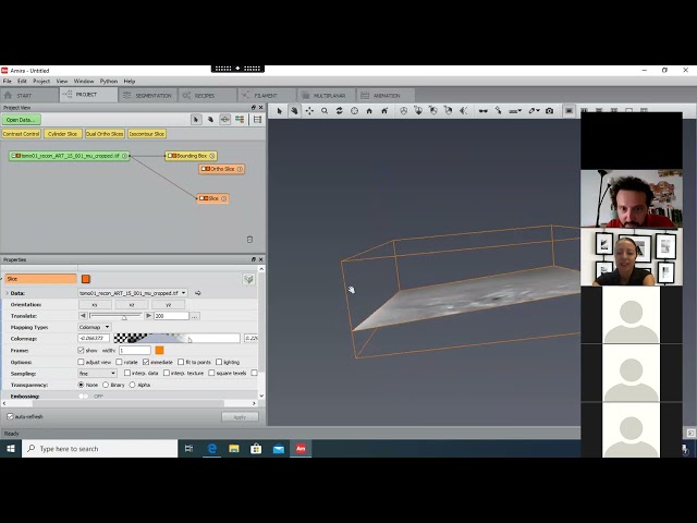
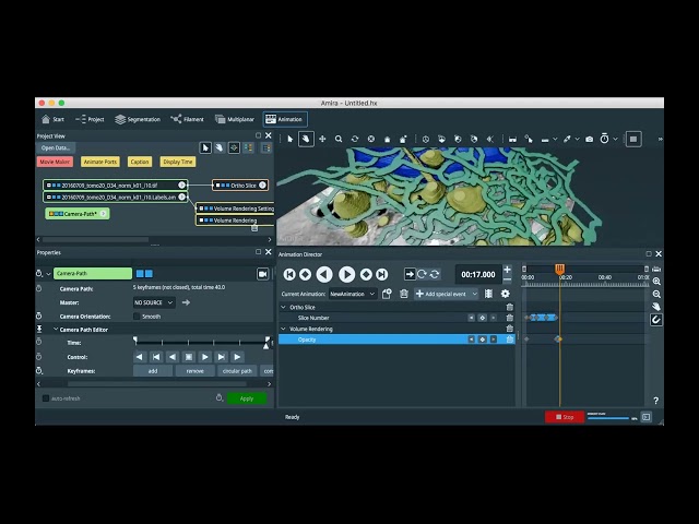
To open volume
To open volume with:
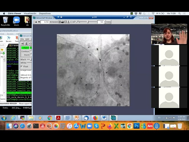
- 3dmod volume.mrc (use Image/XYZ for visualizing all planes)
- fiji/import/mrc leginon
Command line used to go from acquired single tomos txrm stack files to a fully reconstructed stack:
This command line is used to go from acquired single tomos txrm stack files (Sample stack and FlatField stack), into a fully reconstructed stack. Passing through conversion from txrm to hdf5, normalization, deconvolution, alignment and reconstruction volume for processing several topographies in the same folder:
for i in XX; do txrm2deconv 20XXXXXX_tomo"$i".txrm 20XXXXX_tomo"$i"_FF.txrm -zp=25 -e=520 -dx=11 -k=0.05 -t=-1 && ctalignxcorr 20200208_tomo"$i"_norm_deconv_k_0.05.mrc 20200208_tomo"$i"_norm.hdf5 && tomo3d -i *.ali -a *.tlt -o x -S -l 20 -z 700 && trimvol -yz x 20200208_tomo"$i"_3DS20.mrc && rm x; done
for i in 04 05 06 07 08 09; do cd ../tomo$i/ && txrm2deconv 20210519_tomo"$i".txrm 20210519_tomo"$i"_FF.txrm -zp=25 -e=520 -dx=11 -k=0.05 -t=-1 && ctalignxcorr 20210519_tomo"$i"_norm_deconv_k_0.05.mrc 20210519_tomo"$i"_norm.hdf5 && tomo3d -i *.ali -a *.tlt -o x -S -l 30 -z 700 && trimvol -yz x 20210519_tomo"$i"_3DS30.mrc && rm x ; done
Processing for multifocal tomography
1. autoprocessing done in parallel when collecting with macroexecutor “autotomo”: each tomo will be saved in different data_XX folder, normalised hdf5 stacks of each foci and fused (FS) stacks will be made and saved outside the “data_XX” folders:
tomo01-03 (folder)
data_01 (subfolder)
data_02 (subfolder)
data_03 (subfolder)
date_tomo01_E_ZPzPos1_stack.hdf5 (file)
date_tomo01_E_ZPzPos2_stack.hdf5 (file)
date_tomo01_E_ZPzPos3_stack.hdf5 (file)
date_tomo01_E_FS.hdf5 (file)
When FS stack created by ctbio
2. Deconvolution: tomo_deconv 25 520 date date_tomoXX_FS.hdf5 pixel_size K Zsize
default values for FS: K=1/SNR=0.02, Zsize=20 (in microns)
default values for single: K=0.05, Zsize=-1
tomo_deconv 40 520 20190710 XXX_FS.mrc 13 0.1 -1
Deconvolute many FS.mrc in the same folder:
deconv folder 25 520 20190509 px K Zs /beamlines/bl09/controls/user_resources/psf_director
3. -ln(stack.ali) for getting the linear absorption coefficients
4. ctalignxcorr XXX_deconv.mrc XX_norm(FS).hdf5 (hdf5 needed to extract angles)
ctalignxcorr XXX_deconv.mrc 20190430_tomo004_norm.hdf
5. tomo3d -a 20190430_tomo004_norm.tlt -i 20190430_tomo004_norm.ali -S 20
S=SIRT, 20=iterations
Fast tomographic reconstruction on multicore computers
Agulleiro & Fernandez. Bioinformatics 27:582-583, 2011
http://dx.doi.org/10.1093/bioinformatics/btq692
produces “recon_XXX_ali” which is a “xzy” view of the volume
6. to obtain a “xyz” view of the volume: trimvol -yz recon_XXX.ali recon_XXX.ali
Download experimental data
The remotely download of the experiment data for windows could be done following the https://www.cells.es/en/users/your-experiment/after-your-experiment#section-3